Excel 2013 Advanced Formulas and Functions: Boost Productivity With Pro-Level Calculations

Stuck manually updating calculations when your data changes? Array formulas in Excel 2013 let you perform multiple calculations in a single cell—no macros or helper columns required. Unlike traditional formulas, they automatically adjust when referenced ranges update, making them perfect for financial models, dynamic pricing tables, or inventory forecasts.

Use curly braces {} to define arrays (e.g., {=SUM(A1:A10*B1:B10)}) or press Ctrl+Shift+Enter to enter them. They handle operations like multiplying two ranges, finding max/min values across conditions, or even custom logic without VBA. For example, {=IF(COUNTIF(A1:A10,">100")>5,"High Volume","Normal")} dynamically flags high-value transactions in real time.

Financial analysts, inventory managers, and small business owners will love how array formulas eliminate manual recalculations—just update your source data, and results adjust instantly. No more chasing dependencies! ⚡

Frustrated when VLOOKUP refuses to work because your data isn’t sorted left-to-right? The INDEX-MATCH combo is your upgrade path—faster, more flexible, and works with unsorted data without helper columns. Unlike VLOOKUP’s rigid column structure, INDEX-MATCH lets you look up values vertically and horizontally, even across multiple sheets.

Here’s how it works: =INDEX(returnrange, MATCH(lookupvalue, lookup_range, 0)). The MATCH function finds the position of your lookup value, while INDEX retrieves the corresponding result. Need to pull a product price from a separate sheet? No problem. Want to handle partial matches or wildcards? INDEX-MATCH handles it all without the #N/A headaches of VLOOKUP. For large datasets, it’s also 20-30% faster in benchmarks.

Accountants reconciling transactions, inventory managers tracking stock levels, or analysts merging datasets will see immediate gains. Ditch the workarounds and upgrade to a lookup function that actually scales. ⚡

Tired of simple IF statements limiting your spreadsheet logic? Nested IF statements in Excel 2013 let you evaluate multiple conditions in a single formula—perfect for HR approval workflows, dynamic inventory alerts, or multi-tiered project status tracking.

With up to 64 nested IFs (Excel 2013’s limit), you can chain conditions like `=IF(AND(A1>100, B1="Approved"), "Priority", IF(AND(A1>50, B1="Pending"), "Medium", "Low"))`. Use logical operators (AND, OR, NOT) to refine decisions, and wrap results in custom text or values. The formula bar’s auto-indent helps visualize nested structure.

This is your go-to for multi-condition scenarios—like auto-classifying orders by size and region, or flagging overdue tasks with escalation tiers. No VBA required! ⚡

Tired of manually scrubbing messy data in customer records or product lists? Excel 2013’s wildcards and regular expressions (REGEX) let you automate text extraction, validation, and replacement—no programming required. This is your secret weapon for cleaning up inconsistent phone numbers, standardizing product codes, or validating email formats across thousands of rows.

Wildcards like (any sequence) and ? (single character) work out of the box in functions like SEARCH or SUBSTITUTE. For advanced patterns, use Excel’s built-in REGEX support (via Find & Select > Use Wildcards) to match email domains (@.\.com), extract ZIP codes (\d{5}(-\d{4})?), or validate credit card formats. Combine with TRIM, CLEAN, and SUBSTITUTE for a zero-config data-cleaning pipeline.

Marketing teams standardizing lead lists, logistics managers parsing shipment labels, or database admins enforcing format rules will see immediate ROI. No VBA skills needed—just a few clever formulas to transform chaotic text into structured data. ✨

Tired of financial models that assume cash flows arrive like clockwork? XNPV and XIRR handle real-world timing—whether payments are delayed, staggered, or irregular.

Use XNPV to calculate the net present value of cash flows with exact dates (unlike NPV’s fixed intervals), then XIRR to determine the true internal rate of return across uneven schedules. For example, a small business owner tracking quarterly payments with varying dates can now see accurate profitability metrics without manual adjustments.

Accountants and investors will love these functions for audit-ready precision—no more guessing about timing impacts. Perfect for lease analysis, project cash flows, or any scenario where payments don’t follow a predictable pattern. ✨

Tired of spreadsheets crashing or displaying cryptic errors like #DIV/0! or #VALUE! when auditing financial reports or inventory logs? The IFERROR and IS functions act as a safety net, ensuring your data remains clean and professional—even when inputs are unpredictable.

Use IFERROR to replace error messages with custom text (e.g., =IFERROR(A1/B1, "N/A")), while IS functions like ISNUMBER or ISERROR let you test conditions before calculations. Together, they’re ideal for validating data ranges, preventing crashes during bulk imports, or generating error-free reports for stakeholders.

Auditors, accountants, and data analysts will appreciate how these functions maintain data integrity without extra helper columns. Your spreadsheets will run smoother—and look more polished. ✨

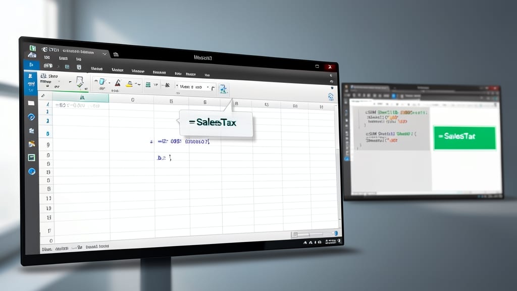
Tired of typing out the same complex formula over and over? User-defined names in Excel 2013 let you assign shortcuts like "=SalesTax" to a formula like =B2*0.0825, saving time and reducing errors. This feature is a game-changer for teams or repetitive tasks where consistency matters.

To create one, go to Formulas > Name Manager and define a name with a formula (e.g., =SUM(B2:B100)/COUNT(B2:B100)). Now, typing =AvgSales instantly calculates the average—no manual entry needed. You can even scope names to specific sheets or workbooks for better organization.

Accountants, inventory managers, or anyone crunching the same data daily will love this zero-config shortcut that keeps spreadsheets clean and error-free. ✨